-
Notifications
You must be signed in to change notification settings - Fork 15
The New Turing Omnibus Chapter 6 Game Trees

Two related algorithms for game playing:
Specifically for games that:
- Are zero-sum (viz. the win and loss of players balance each other out, e.g. one player wins, the other loses);
- Have perfect information (viz. the computer can see all players’ moves, nothing is hidden).
Minimax is an algorithm for minimising the maximum possible loss (assuming your opponent will make the best move possible and always attempting to minimise your own loss).
Alpha-beta pruning is a technique used to optimise the Minimax algorithm.
(Not in the chapter but might be useful to set the scene.)
Could represent a game from a single player’s perspective as a tree with the root node as the starting board and then all possible moves as branches with each level alternating between players. If the game is simple enough, could use the British Museum algorithm to solve: calculate all possible moves and choose the move that is most likely to result in a win for the player.
In reality, most games have trees far too large to make this computationally efficient (or even possible). Chess has around 10120 leaf nodes which would take longer than the age of the universe in nanoseconds multiplied by the number of atoms in the universe to evaluate.
Good way to size a game is to look at its branching factor b (how many branches does a node have) and its depth d (how many levels does the tree have to its terminal nodes). As our strategy relies on evaluating each terminal node (to determine whether it is a win for the player or not), we can use the number of terminal nodes as a measure of our work.
The number of terminal nodes in a tree is given by bd. So for the following tree:
      o
   /     \
  o       o
 / \     / \
o   o   o   o
b = 2, d = 2, so the number of terminal nodes is bd = 22 = 4.
MAX        o
        /     \
MIN    o       o
      / \     / \
     2   7   1   8
Imagine a simple game where the player wants to achieve the maximum score and their opponent wants to achieve the minimum score.
Starting at the terminal nodes, we choose the minimum value as it benefits the opponent (which wants the smallest possible number):
MAX        o
        /     \
MIN    2       o
      / \     / \
     2   7   1   8

MAX        o
        /     \
MIN    2       1
      / \     / \
     2   7   1   8
We then choose the maximum value for the player:
MAX        2
        /     \
MIN    2       1
      / \     / \
     2   7   1   8
This shows that the best move for the player to make would be to go the left. Note that this doesn’t give the player the maximum possible value in the game (8) but actually represents the adversarial nature of the game whereby the opponent will want to win also.
A Ruby example of the game above might be implemented like so:
def minimax(node, depth, maximizing_player)
  return node.value if depth.zero? || node.terminal?

  if maximizing_player
    best_value = -Float::INFINITY
    node.children.each do |child|
      value = minimax(child, depth - 1, false)
      best_value = [best_value, value].max
    end
  else
    best_value = Float::INFINITY
    node.children.each do |child|
      value = minimax(child, depth - 1, true)
      best_value = [best_value, value].min
    end
  end

  best_value
end

class Node
  attr_reader :value, :children

  def initialize(value: nil, children: [])
    @value = value
    @children = children
  end

  def terminal?
    children.empty?
  end
end

origin = Node.new(
  children: [
    Node.new(
      children: [
        Node.new(value: 2),
        Node.new(value: 7)
      ]
    ),
    Node.new(
      children: [
        Node.new(value: 1),
        Node.new(value: 8)
      ]
    )
  ]
)

puts minimax(origin, 2, true)
#=> 2The deeper we can go in the game tree the better informed our move so it would be beneficial to optimise which parts of the tree we need to explore. Ideally, we wouldn’t need to evaluate all terminal nodes, just ones that are relevant to us.
If we evaluate each terminal in turn, we can actually avoid exploring entire branches of the tree like so:
MAX        o
        /     \
MIN    o       o
      / \     / \
     2   o   o   o
The first value we evaluate is 2 so the minimising opponent immediately knows that it will pick a value that is less than or equal to 2 (as it will pick the smallest possible value):
MAX        o
        /     \
MIN   <=2      o
      / \     / \
     2   o   o   o
Upon evaluating the next terminal, we see that the value must be 2 as 7 is larger than 2 and therefore not a better move.
MAX        o
        /     \
MIN    2       o
      / \     / \
     2   7   o   o
With that, the maximiser knows it must pick a value greater than or equal to 2 to win:
MAX       >=2
        /     \
MIN    2       o
      / \     / \
     2   7   o   o
We then evaluate the next terminal:
MAX       >=2
        /     \
MIN    2       o
      / \     / \
     2   7   1   o
The minimiser knows it will pick a value less than or equal to 1:
MAX       >=2
        /     \
MIN    2     <=1
      / \     / \
     2   7   1   o
Now the maximiser knows that if it goes to the right, it can’t do better than 1 (as the minimiser will result in a value that is at most 1) and it knows if it goes left it can get at least 2 so it can exclude that entire branch of the tree from the calculation.
MAX       2
        /
MIN    2
      / \
     2   7
An example of Minimax with alpha-beta pruning in Ruby for the above game is as follows:
def alphabeta(node, depth, a, b, maximizing_player)
  return node.value if depth.zero? || node.terminal?

  if maximizing_player
    value = -Float::INFINITY
    node.children.each do |child|
      value = [value, alphabeta(child, depth - 1, a, b, false)].max
      a = [a, value].max
      break if b <= a
    end
  else
    value = Float::INFINITY
    node.children.each do |child|
      value = [value, alphabeta(child, depth - 1, a, b, true)].min
      b = [b, value].min
      break if b <= a
    end
  end

  value
end

class Node
  attr_reader :value, :children

  def initialize(value: nil, children: [])
    @value = value
    @children = children
  end

  def terminal?
    children.empty?
  end
end

origin = Node.new(
  children: [
    Node.new(
      children: [
        Node.new(value: 2),
        Node.new(value: 7)
      ]
    ),
    Node.new(
      children: [
        Node.new(value: 1),
        Node.new(value: 8)
      ]
    )
  ]
)

puts alphabeta(origin, 2, -Float::INFINITY, Float::INFINITY, true)
#=> 2Not discussed in detail in the chapter, this is sometimes referred to as a heuristic evaluation function, taking the state of the game and determining whether a player is advantaged or not and assigning a numeric value (e.g. a particular “position” may be measured as +7 for the red player if it is advantageous).
This will be different for each game and there may be different heuristics for different games (how can you measure how advantageous a particular position is in Chess?)
Simplest possible implementation is to only use the position evaluator on the terminal leaf nodes of the game tree: assign values for win (e.g. 1), lose (e.g. -1) or draw (e.g. 0) with respect to the player and the Minimax algorithm can still work using only that. More complicated games (e.g. with trees too large to fit in memory) will require the evaluator to run on intermediate nodes.
- 6. Search: Games, Minimax, and Alpha-Beta, MIT OpenCourseWare;
- Let’s Learn Python #21 - Min Max Algorithm, Trevor Payne;
- An Exhaustive Explanation of Minimax, a Staple AI Algorithm, Daniel Higginbotham;
- Tic Tac Toe: Understanding The Minimax Algorithm, Jason Fox.
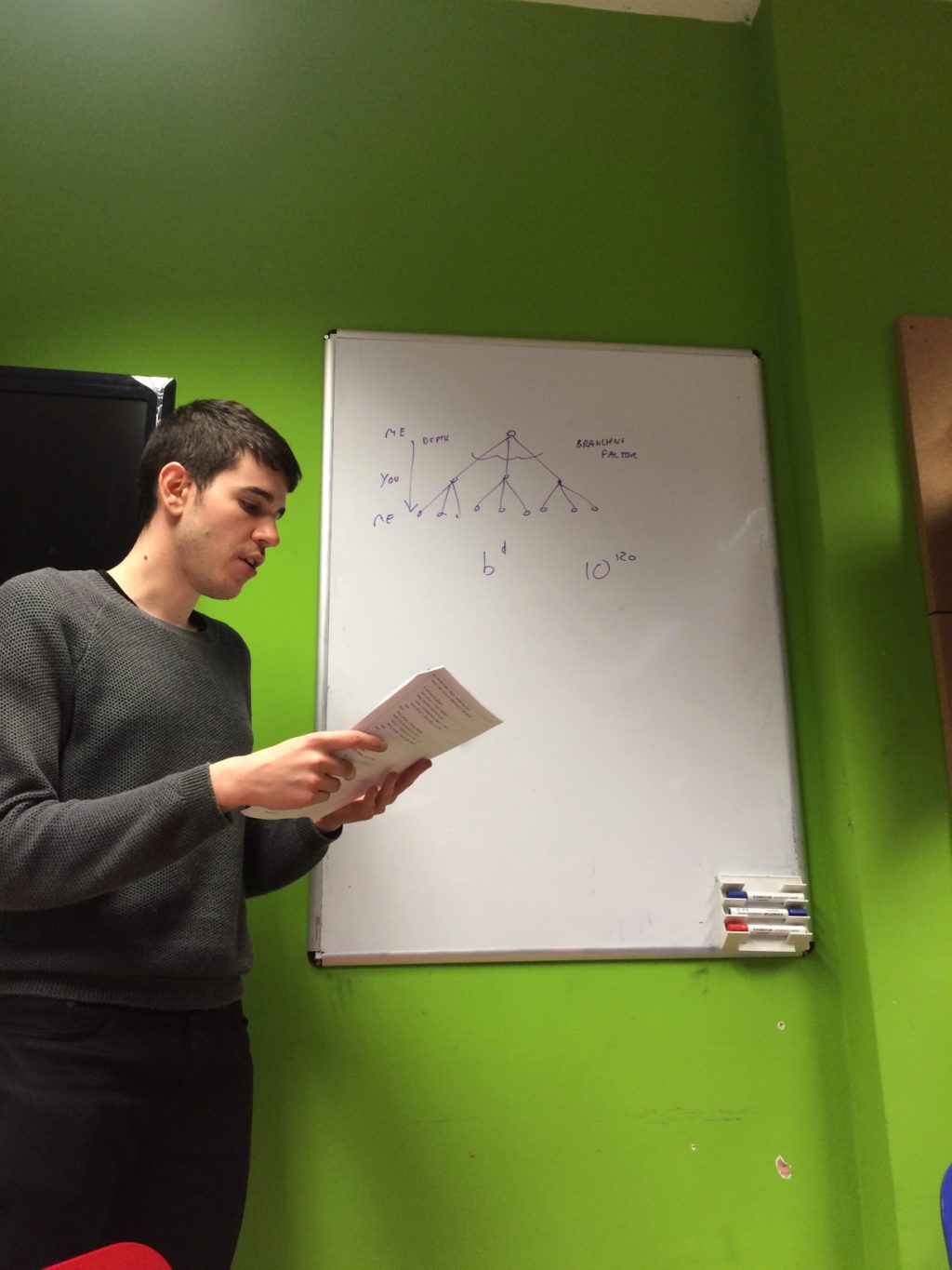
Paul acted as shepherd of this meeting and talked through the notes above, explaining the two algorithms in detail using a simple example separate from the chapter's checkers example.
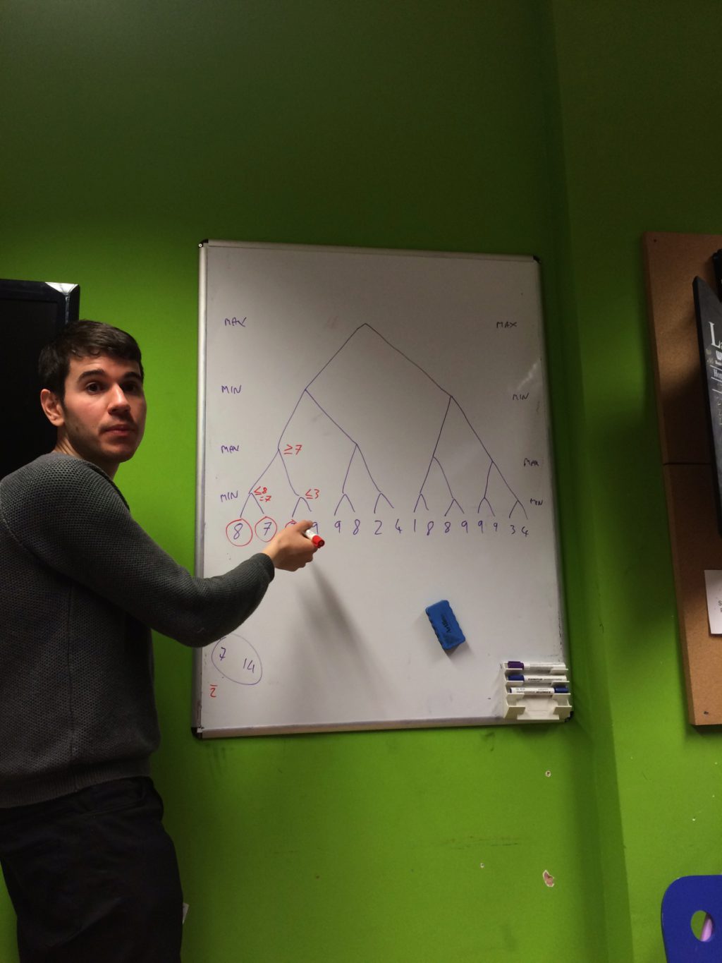
We discussed the properties of the static evaluation function used to rank moves and how looking ahead deeper in the tree apparently simplifies these functions (e.g. in chess, if you can look ahead far enough, all that matters is piece count). We convinced ourselves this might be intuitive given the ultimate depth (viz. the endgame), all that really matters is a win, loss or draw.
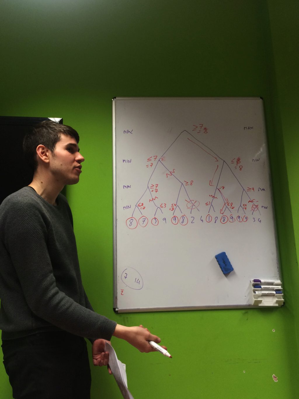
With the first hour complete and everyone now familiar with the algorithm, we decided to mob program a noughts and crosses game in Ruby.
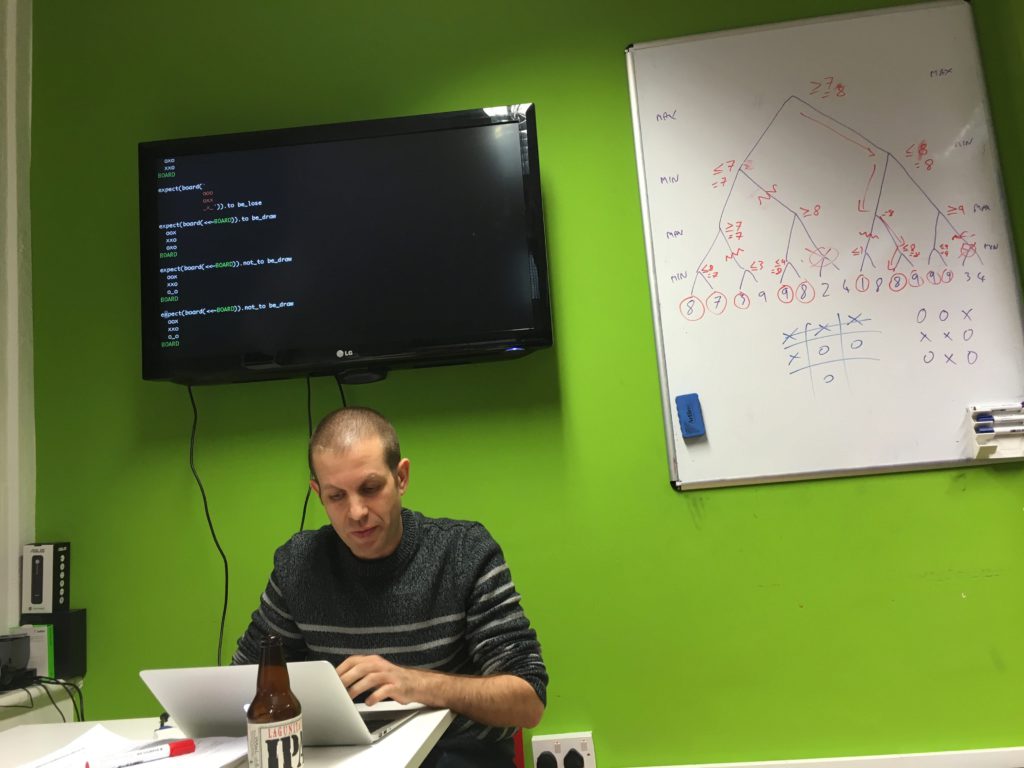
Tom took to the keyboard and began by writing some specs for our program.
We decided to represent a given board as a two-dimensional array of either xs, os or _s and used a convenience function to build these boards out of strings like the following:
board(<<EOF)
___
_x_
o__
EOF
We then made it possible for each board to determine whether it was won, lost or drawn and derived a score from that (1, -1 or 0 respectively). This gave us the first part of the input to the Minimax algorithm (the evaluation function) so we then moved onto generating the game tree.
Given a board, we added a method to generate the next possible moves, giving us the second part of the algorithm.
With these two things, we could then enhance our scoring to recursively descend the tree and return the highest score. We can then use this to pick the appropriate move for a player by ensuring that we alternated between scoring moves for ourselves and for our opponent (the min and max part of the algorithm).
With this, we play a game on the command line and some of us were enthralled by this epic battle between Computation Club and the artificial intelligence we had wrought.
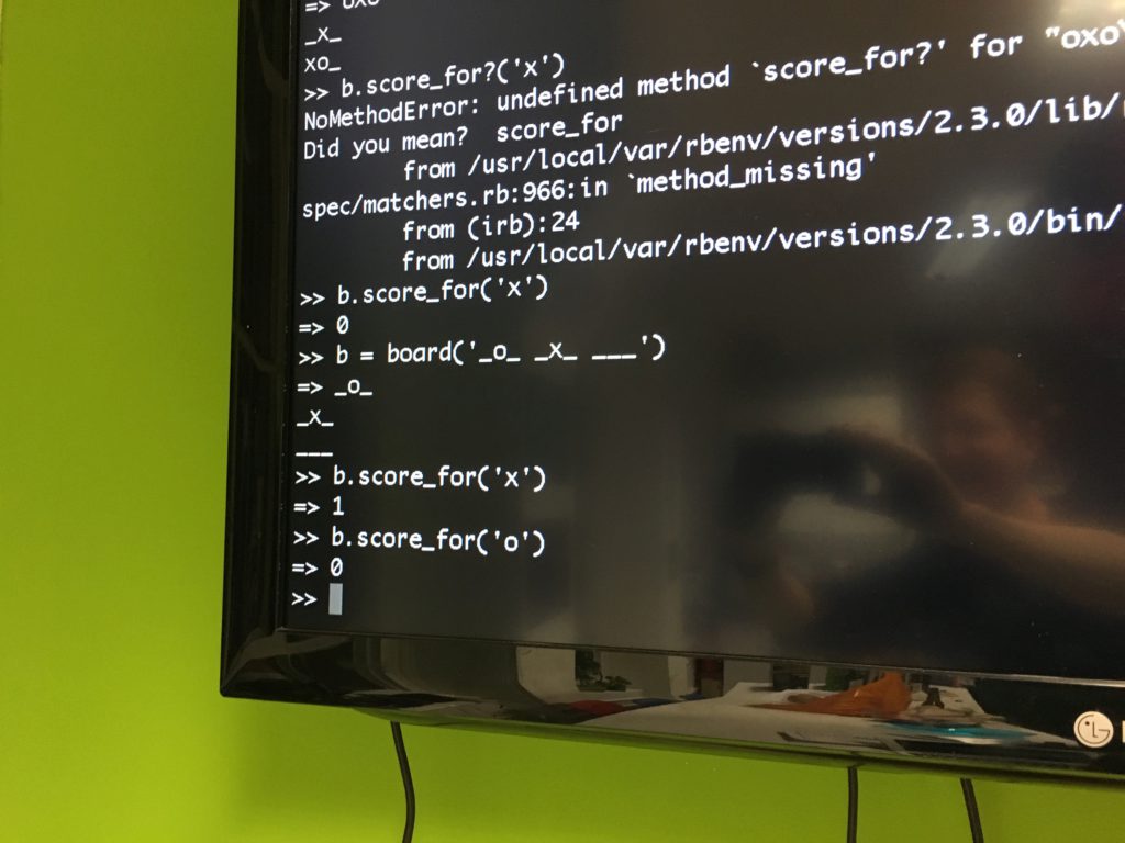
Interestingly, we explored the behaviour of the game when we initially disadvantaged the opponent by placing a o in one of the corners of the board and saw how it immediately concluded we would win and it would lose.
You can find the code on GitHub and we were interested to discover that the algorithm was very slow when given a totally blank board. We wondered whether implementing alpha-beta pruning would improve this but, in the meantime, we should made sure to start the game with an initial move played.
As we slightly ran over, we held a brief retrospective in the pub:
- Feelings were overall very positive with some saying this was one of our best meetings from The New Turing Omnibus;
- Again, we placed a huge value on having a shepherd for the meeting;
- As this has been come up several times now, we agreed that we should always prefer to hold meetings with one member doing some preparation (even if only watching some lectures on the topic, etc.) and, if no one is available, we flag this up as early as possible so that we can adjust our approach to the meeting;
- In order to give shepherds as much preparation time as possible, we decided to closing voting as soon after the meeting as possible to ideally give members two weekends in which to prepare;
- We also noted that some of our best meetings have been when we use the chapter as a springboard for a topic: almost all of Paul's materials for this meeting came from an MIT lecture and not from the book itself but it was still valuable;
- With this in mind, we decided to relax the CfP process and our approach to the book so that we can discuss wider topics in Computation and not be afraid to go "off-book".
Thanks to Leo and Geckoboard for hosting, to Paul for his exceptional preparation and shepherding, and to Tom for commandeering the keyboard while we shouted bits of Ruby.
- Home
- Documentation
- Choosing a Topic
- Shows & Tells
- Miscellaneous
- Opt Art
- Reinforcement Learning: An Introduction
- 10 Technical Papers Every Programmer Should Read (At Least Twice)
- 7 More Languages in 7 Weeks
- Lua, Day 1: The Call to Adventure
- Lua, Day 2: Tables All the Way Down
- Lua, Day 3
- Factor, Day 1: Stack On, Stack Off
- Factor, Day 2: Painting the Fence
- Factor, Day 3: Balancing on a Boat
- Elm, Day 1: Handling the Basics
- Elm, Day 2: The Elm Architecture
- Elm, Day 3: The Elm Architecture
- Elixir, Day 1: Laying a Great Foundation
- Elixir, Day 2: Controlling Mutations
- Elixir, Day 3: Spawning and Respawning
- Julia, Day 1: Resistance Is Futile
- Julia, Day 2: Getting Assimilated
- Julia, Day 3: Become One With Julia
- Minikanren, Days 1-3
- Minikanren, Einstein's Puzzle
- Idris Days 1-2
- Types and Programming Languages
- Chapter 1: Introduction
- Chapter 2: Mathematical Preliminaries
- Chapter 3: Untyped Arithmetic Expressions
- Chapter 4: An ML Implementation of Arithmetic Expressions
- Chapter 5: The Untyped Lambda-Calculus
- Chapters 6 & 7: De Bruijn Indices and an ML Implementation of the Lambda-Calculus
- Chapter 8: Typed Arithmetic Expressions
- Chapter 9: The Simply-Typed Lambda Calculus
- Chapter 10: An ML Implementation of Simple Types
- Chapter 11: Simple Extensions
- Chapter 11 Redux: Simple Extensions
- Chapter 13: References
- Chapter 14: Exceptions
- Chapter 15: Subtyping – Part 1
- Chapter 15: Subtyping – Part 2
- Chapter 16: The Metatheory of Subtyping
- Chapter 16: Implementation
- Chapter 18: Case Study: Imperative Objects
- Chapter 19: Case Study: Featherweight Java
- The New Turing Omnibus
- Errata
- Chapter 11: Search Trees
- Chapter 8: Random Numbers
- Chapter 35: Sequential Sorting
- Chapter 58: Predicate Calculus
- Chapter 27: Perceptrons
- Chapter 9: Mathematical Research
- Chapter 16: Genetic Algorithms
- Chapter 37: Public Key Cryptography
- Chapter 6: Game Trees
- Chapter 5: Gödel's Theorem
- Chapter 34: Satisfiability (also featuring: Sentient)
- Chapter 44: Cellular Automata
- Chapter 47: Storing Images
- Chapter 12: Error-Correcting Codes
- Chapter 32: The Fast Fourier Transform
- Chapter 36: Neural Networks That Learn
- Chapter 41: NP-Completeness
- Chapter 55: Iteration and Recursion
- Chapter 19: Computer Vision
- Chapter 61: Searching Strings
- Chapter 66: Church's Thesis
- Chapter 52: Text Compression
- Chapter 22: Minimum spanning tree
- Chapter 64: Logic Programming
- Chapter 60: Computer Viruses
- Show & Tell
- Elements of Computing Systems
- Archived pages